For some time now I wanted to find a way where my personal projects will be well documented, such that I can have an organized code base and notes on the topic I was exploring. Typically I find writing notes tedious, and for that reason I’ve decided to turn this into more of a free-style blog post. This one will hopefully be first of many, and as such I hope thier quality will be better and better.

The first section is devoted to auto-encoder objectives in general: reconstruction loss, KL loss, adversarial and perceptual loss, if you are well acquainted with these fell free to jump directly into section two that focuses on currently the most popular design choices and optimization tricks for modern audio auto-encoders.

If you want to see a nice implementation of the set-up described below feel free to checkout my repo here.

1. Auto-encoders in General

1.1. 🚪 Introduction 🚪

Auto-encoders are a type of neural network architecture composed of two, often symmetrical networks called the encoder $\mathcal{E}$ and the decoder $ \mathcal{D} $ each with their own sets of parameters $ \theta $ and $ \psi $ respectively.

In its simplest implementation the networks are trained to be the inverse to one another, where the encoder processes the data into latent features, next the decoder takes the latent features and tries to reconstruct the input data from the encoder latents. To enforce this a reconstruction loss is used, often in the form of a L2 distance

\[\mathcal{L}_{rec}(\psi,\theta) = ||x - \mathcal{D_\psi}(\mathcal{E_\theta(x)}) ||_2\]

We might be inclined to believe that this should be enough for the encoder to produce a meaningful set of features representing the most important properties of data, all the while compressing it a sufficient amount. The latter is achieved simply by architecture design choices such as down sampling layers, but is almost certainly guaranteed to fail.

The reason for that is that nothing is forcing the latent space to be smooth, and if nothing is enforcing said smoothness the model will follow the path of least resistance during optimization.

One of two things can happen, the model either severely over-fits and memorizes the data as a look-up table in the latent space, i.e. each example gets placed in an arbitrary latent point that the decoder can reconstruct, but besides those few points the rest of the latent space is useless. A slightly smaller issue is not that the model over-fits, rather it creates small clouds in the latent space. In terms of data distribution in the latent space this means the model learns localized regions of very low variance that are very far a part. Overall the latent space will have very high variance because of that.

How do we fix this? Enter the variational auto-encoder (VAE)!

1.2. 🔔 KL-Divergence Loss 🔔

Instead of only forcing the auto-encoder to produce good reconstructions, we add another term to the loss, the so-called Kullback-Leiber divergence, it is a measure of how different two distributions are. The idea is that if the model produces some ugly distribution in the latent space, why not force it to take a form of a more well behaved probability distribution, and what is more well behaved than a Gaussian?

To that end we assume that the desired data distribution in the latent space is normal $ p(z) = \mathcal{N}(0,1) $. Furthermore, we want to enforce that the distribution that the model produces $ q_\phi(z) = \mathcal{N}(\mu_\phi(z),\sigma_\phi(z)^2) $ is also Gaussian. This yields a simplified version of the KL divergence loss given by the equation (1)

\[\mathcal{L}_{KL} = \sum_z q_\phi(z) \log\frac{q_\phi(z)}{p(z)} =\Big\{\mathrm{Gaussian}\Big\} = \frac{1}{2}\sum_{j=1}^{D}(1 + \log \sigma_j^2 - \mu_j^2 - \sigma_j^2) \quad(1)\]

This loss will enforce several things

It will reduce the overall variance of the latent representations forcing the model to abandon the strategy of lumping data into distant low-variance lumps.
Since the overall variance of the latents is penalized it will confine the data into a smaller part of the overall latent space ensuring a higher degree of smoothness.
Bonus points if we now wish to sample novel data we can simply sample from a Gaussian distribution in the latent space and pass that latent vector to the decoder.

1.3. 🎩 Reparametrization trick 🎩

The astute reader will notice that in order to calculate the KL loss we need access to the variance and mean of the latent data. To make things worse this needs to be calculated at every optimization step, which makes this at best computationally inefficient at worst impossible to back-propagate against. To solve this Kingma and Welling [2], introduce the reparametrization trick.

They say instead of the encoder $ \mathcal{E}$ producing latents directly, rather it produces the mean and variance of the data

\[\mathcal{E}_\theta(x) = (\mu_\theta(x),\sigma_\theta(x) )\]

The actual latent vector is now retrieved by sampling from the following distribution

\[z = \mu_\theta(x) + \sigma_\theta(x) \cdot\epsilon \quad \epsilon\sim \mathcal{N}(0,1) \quad (2)\]

It turns out this simple trick makes the calculation of the KL-loss and its gradients tractable.

1.4. ⚖️ It’s still not enough! Adversarial and Perceptual loss ⚖️

During, the olden days of generative modeling the two main approaches were auto-encoders and the generative adversarial networks (GANs). Auto-encoders provided meaningful latents, some degree of interpretability, and an ease of training, but GANs had crisper data reconstructions. Most notably in the case of image generation, the images produced with VAEs were blurry, and the ones produced by GANs were crisp.

Nowadays, we require the best of both worlds - the neat and interpretable latent space of VAEs and the high quality reconstructions provided by GANs. To this end modern auto-encoder training procedures include an adversarial and perceptual loss term.

1.4.1. 🥊 Adversarial Loss 🥊

The real data $x$ and the reconstructed data $ \hat{x} = \mathcal{D}(\mathcal{E(x)}) $ are passed to the discriminator model $ \Phi $, which is trained to distinguish between real and reconstructed (fake) data. Furthermore, the auto-encoder is also trained to fool the discriminator. These two networks are optimized independently (each with its own optimizer) and trained in tandem.

The discriminator loss is given by equation (3)

\[L_{Adv}^{\Phi} = -\mathbb{E}_{x \sim P_{data}} [\log \Phi(x)] - \mathbb{E}_{x \sim P_{data}} [\log (1 - \Phi(\mathcal{D}(\mathcal{E}(x))))]\quad (3)\]

While the auto-encoder adversarial loss is given by equation (4)

\[L_{Adv}^{AE} = -\mathbb{E}_{x \sim P_{data}} [\log \Phi(\mathcal{D}(\mathcal{E}(x)))]\quad (4)\]

1.4.2. 🔎 Perceptual Loss 🔎

As a last component of the loss there is also the perceptual loss. It turns out the L2 reconstruction loss is too local, and does not enforce reconstruction realism to a high enough degree, since it is calculated in a pixel-wise manner it cannot capture more global perceptual features.

To this end we try to squeeze out a bit more juice from out discriminator. Typically these discriminators are built in such a way that they sequentially increase their receptive field, and if trained properly each layer produces higher-order perceptual features.

\[\Phi = \varphi_1 \circ\varphi_2...\circ\varphi_n\]

In practice this is calculated by taking the intermediate outputs from each layer of the discriminator $\varphi_l$, for both original $x$ and reconstructed data $\hat{x}$ and calculating the L2 distance between the two.

\[\mathcal{L}_{per} = \sum_{l\in\mathrm{layers}} ||\varphi_l(x) - \varphi_l(\hat{x})_l ||_2 \quad (5)\]

Modern auto-encoders require all of these ingredients to fully function, and now that we’re fully equipped with the terminology and intuition we can further discuss how to apply these ideas in audio.

2. Modern Audio Auto-encoders

2.1. 🌊 Waveform or Spectrogram?🌊

In this section I will explain the architectural and optimization choices for modern audio auto-encoders. We use the term modern here mainly for an architecture presented in papers [4,5,6].

A typical approach in modeling audio will allow the model to process either spectrograms or mel-spectrograms [8, 9, 10] rather than raw audio, and for some time it seemed that models that tried to process raw waveforms performed significantly worse than their frequency domain counterparts. The spectrogram representation is not without its flaws either. As one moves from lower to higher frequencies the scale of the features becomes smaller and smaller, this often rendered computer-vision-like approaches unsuccessful and required tricks such as band splitting [10,11].

The mel-spectrogram scale does allow for the use of computer vision techniques in a more off-the-shelf manner. Sander Dieleman gives a nice explanation as to why that is in his blog, which I highly recommend, but the gist of it is that the frequencies present in images and mel-spectrograms (2D Fourier transforms of images or mel-spectrograms) follow the same power law.

Below you can see the radially averaged power spectral density, or RAPSD for a 2D Foruier transform of an image, spectrogram, and mel-spectrogram. The RAPSD graphs are in log-scale where the presence of a power law in image and mel-spectrograms are evident.

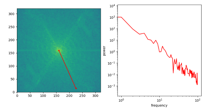
**FIG 1:** From Sander’s blog, on the left is an 2-D Fourier transform of an image, and the frequencies are taken across the red line, on the right the frequency power along the red line is displayed in log-log scale. Even here a power law is evident.

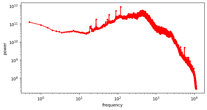
FIG 1: From Sander’s blog, on the left is an 2-D Fourier transform of an image, and the frequencies are taken across the red line, on the right the frequency power along the red line is displayed in log-log scale. Even here a power law is evident.

**FIG 2:** RAPSD for ordinary spectrogram, power law is not present.

FIG 2: RAPSD for ordinary spectrogram, power law is not present.

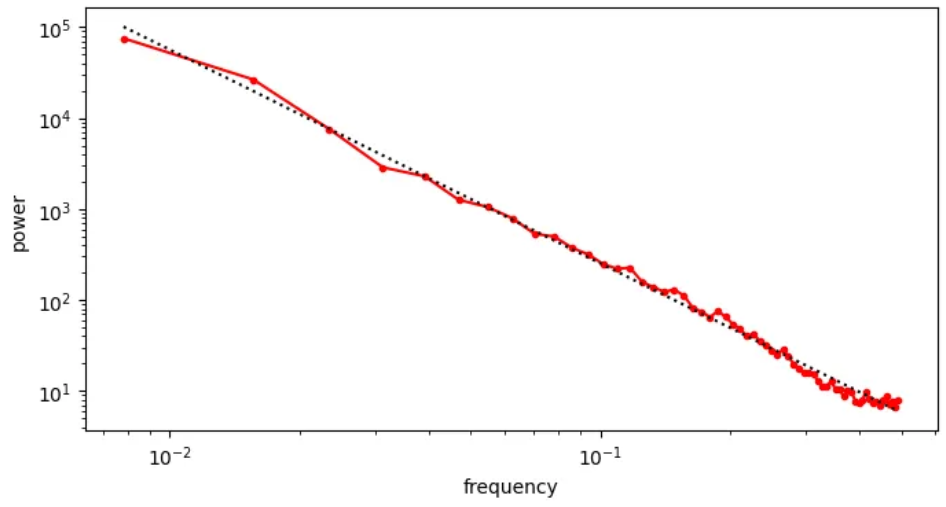
**FIG 3:** RAPSD for mel-spectrogram, the power law again becomes apparent.

FIG 3: RAPSD for mel-spectrogram, the power law again becomes apparent.

Why not work with mel-spectrograms then? The reason is that they perform a great deal of frequency compression in the form of band averaging. This sometimes does not present an issue when one is dealing in classification tasks, or in voice reconstruction, where a high frequency resolution is not essential. However, when dealing with all sorts of audio, including music mel-spectrograms prove less then ideal.

2.2. 🗼 Architecture Well Suited For a Waveform 🗼

It turns out that the wavefrom representation does not suffer from varying scale problem we’ve encountered with spectrograms, and unlike mel-spectrograms they do not compress the data. With all of this in mind it turns out that the humble 1-D convolution is enough to process a waveform. ver tricks. Currently the most best models with regards to reconstruction quality, audio compression and downstream utility I have found are the Encodec [5], Descript Audio Codec (DAC) [6] and Oobleck (Stability-AI) [5]. While all three models build on each other and, have certain differences and relative improvements, at their core is a very similar design almost entirely comprised of cleverly implemented of 1-D convolutional layers.

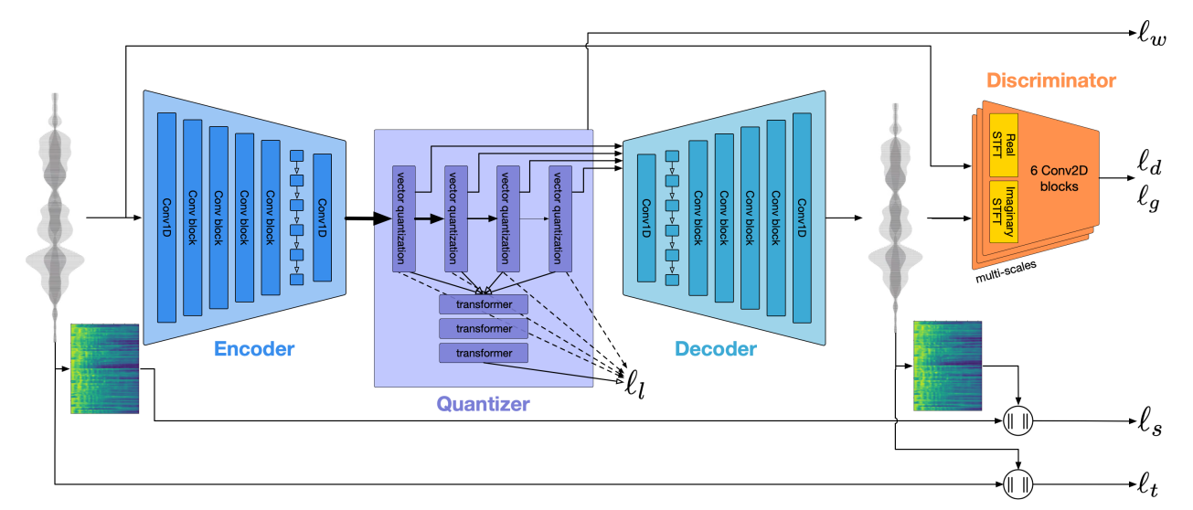
Fig 4: EnCodec Model Architecture [5]: The model processes raw waveforms using a series of 1-D convolutional layers and occasionally a LSTM layer. In this instance the bottleneck layer introduces vector quantization, which the authors of [4,6] often replace with their own latent space reguralization, for instance the stable-audio-open VAE uses the principles of VAE and KL divergence mentioned in sections 1.2 and 1.3. Multiple losses are calculated ,most notably waveform and spectrogram reconstruction losses, adversarial losses and feature matching losses.

In order to capture the highly auto-correlated waveform samples the encoder and decoder blocks rely on dilated ResidualUnits, the motivation is to stack several of these with a wide kernel size (usually 7), and progressively larger dilations (1,3,9). These combine local features present in non dilated kernels and features with a higher receptive field in the case of dilated features.

class ResidualUnit(nn.Module):
    def __init__(self, channels: int, kernel_size: int = 7, dilation: int = 1):
        super().__init__()
        padding = ((kernel_size - 1) * dilation) // 2
        self.block = nn.Sequential(
            Snake(channels),
            WNConv1d(
                channels, channels, kernel_size, dilation=dilation, padding=padding
            ),
            Snake(channels),
            WNConv1d(channels, channels, kernel_size=1),
        )

    def forward(self, x: torch.Tensor) -> torch.Tensor:
        return x + self.block(x)

The EncoderBlock is built from these ResidualUnits , followed by a downsampling layer in the form of a strided convolution.

class EncoderBlock(nn.Module):
    def __init__(
        self,
        in_channels: int,
        out_channels: int,
        stride: int = 2,
        kernel_size: int = 7,
        dilations: List[int] = [1, 3, 9],
    ):
        super().__init__()
        self.res_units = nn.Sequential(
            *[ResidualUnit(in_channels, kernel_size, dilation=d) for d in dilations]
        )
        self.downsample = nn.Sequential(
            Snake(in_channels),
            WNConv1d(
                in_channels,
                out_channels,
                kernel_size=2 * stride,
                stride=stride,
                padding=stride // 2,
            ),
        )

    def forward(self, x: torch.Tensor) -> torch.Tensor:
        return self.downsample(self.res_units(x))

Example: With 4 EncoderBlocks and stride sizes of [2, 4, 4, 8] we can achieve a x256 compression in sample length!

Lastly, the decoder consists of practically the same components in the reversed order, with the exception that instead of downsampling we now upsample with a transposed convolution layer.

class DecoderBlock(nn.Module):
    def __init__(
        self,
        in_channels: int,
        out_channels: int,
        stride: int = 2,
        kernel_size: int = 7,
        dilations: List[int] = [1, 3, 9],
    ):
        super().__init__()
        self.upsample = nn.Sequential(
            Snake(in_channels),
            WNConvTranspose1d(
                in_channels,
                out_channels,
                kernel_size=2 * stride,
                stride=stride,
                padding=stride // 2,
            ),
        )
        self.res_units = nn.Sequential(
            *[ResidualUnit(out_channels, kernel_size, dilation=d) for d in dilations]
        )

    def forward(self, x: torch.Tensor) -> torch.Tensor:
        return self.res_units(self.upsample(x))

Stack several of these layers in the correct order and you have your architecture… But wait! What are the WNConv1d and WNConvTranspose1d, and what is a Snake function?

2.2.1. 🏋️‍♂️ Weight Normalized Layer 🏋️‍♂️

A typical linear layer looks something like this $y = W x + b$ where $W$ and $b$ are the weights and biases of the layer, if we focus only on the weights, a weight normalized linear layer tranformation would instead be parametrized in the following way $y = \frac{g\cdot W}{||W||}x + b$ Now instead of learning the direction and the norm of the the linear transform we separate these two into separate parameters, $ \frac{W}{||W||}$ accounts for the direction of the transform and the $g$ is the learnable norm of the transform, Salimas and Kingma [12] show how this approach speeds up the convergence of the training and that the learned norms are not mini-batch dependent as is the case with batch-normalization.

This can be applied to any layer that can be represented as a linear transform, and as it so happens convolutions and transposed convolutions are just such layers.

2.2.2. 🐍 The Snake Activation Function 🐍

Picking the non-linearity in deep learning models usually involves appeals to intuition, adherence to universal approximation theorems of questionable generalization, and empirical experience. Nevertheless, the list of nonlinear activation functions seems ever growing, and regardless of the cynicism displayed in the first sentence, there are good reasons for exploring novel activation functions most notably that different activation functions are not equally well suited for different types of data.

In that tone Ziyin et al. [7] found that any network with $ \tanh $ or $ \mathrm{ReLU}$ activation cannot extrapolate periodic functions, and although I’ve haven’t found sources proving such properties for other nonlinearities that are $\tanh$-like or $\mathrm{ReLU}$-like: $\mathrm{SiLU}$, $\mathrm{GeLU}$, $\mathrm{Sigmoid}$ etc.

This issue with periodic functions extends to highly oscillating functions, and therefore Ziyin et al. [7] propose the Snake activation function

\[\mathrm{Snake}_a(x) = x + \frac{1}{a^2}\sin^2(ax)\]

Here ‘$a$’ can either be set to a constant scalar and/or vector or a learnable scalar and/or vector, indeed Encodec [5], and Oobleck [4] models with Snake activations (with learnable vector parameters) prove superior to $\mathrm{ReLU}$-like and $\tanh$-like counterparts.

2.2.3. 🍾 The Bottleneck Layer 🍾

Besides the Encoder and Decoder, each of these auto-encoders has a devoted layer and logic to reguralize or further process the latent space. A set of layers and techniques used for this is called the bottleneck layer. And depending on the task at hand one might decide for various different bottlenecks. For instance, the Oobleck auto-encoder present in Stable-Audio-Open [4] utilizes only the KL-loss as a reguralization, i.e. its calculates the mean and log-variance of the latens for a given input and forces the latent distribution to be more Gaussian, as described in section 1.2. This type of reguralization is useful for making a well behaved latent space, that can be used in downstream tasks such as generation, style mixing, anomaly detection or specific to music stem separation.

On the other hand, the Encodec and DAC models [5,6] attempt to reguralize the latent space by quantizing the latent vectors via a code-book of fixed size, a schematic diagram is shown in Fig 4. These currently considered essential in tasks where audio compression is the prime priority.

2.3. 🦍 🐅 🦭 Discriminator Zoo 🦍 🐅 🦭

One final missing peace needs to be explained in the context of high-quality audio auto-encoders, and that is the role of Discriminators. Their use is necessitated by the fact that each of the aforementioned losses work in an extremely local fashion. The L2 reconstruction loss is essentially a pixel-wise loss, both in the time and frequency domain, the KL loss cares not for perceptual quality only that the latent space is well behaved.

Discriminator models are brought in to mitigate these issues by doing the following

Learning to distinguish real from generated data, in tandem with the generator.
They generate higher-order perceptual features that are manifest by their layer activations.

They are especially useful in decoder-fine-tuning when we only care about reconstruction quality, by using discriminators the decoder is forced to to remove typical audio artifact such as a metallic sound. In contrast to original GAN models, here we use a whole ensamble of discriminators each taylored to focus on specific type of perceptual features.

Typical discriminators are the following:

Spectrogram Discriminator (Single Resolution and Multi Resolution)
Multi Scale Discriminators
Period and Multi-Period Discriminators 💡 It is worth noting that these discriminators need not be large, especially in the case of multi-resolution and multi-period discriminators, since their goal is to focus on a subset of features present in the training data.

2.3.1. 🐊 Multi-Resolution Spectrogram Discriminator 🐊

Most prominent discriminators are Spectrogram discriminators, the idea is that we calculate a spectrogram with $N$ frequencies and treat it as an image. This is passed to a convolutional discriminator that utilizes rectangular kernels instead of square ones, and dilation. It is trivial to extend this to a multi-resolution discriminator by simply using an ensamble of these with a varying number of Fourier frequencies. A code example of a single-resolution discriminator is given below, note that for each layer its activations are stored in a feature-map list for later use.

class DiscriminatorSTFT(nn.Module):
    """
    Single STFT-based discriminator operating at one scale.

    Processes complex-valued STFT (real and imaginary parts concatenated)
    with 2D convolutions in time-frequency domain.
    """

    def __init__(
        self,
        filters: int = 32,
        in_channels: int = 1,
        n_fft: int = 1024,
        hop_length: int = 256,
        win_length: int = 1024,
        kernel_size: Tuple[int, int] = (3, 9),
        dilations: List[int] = [1, 2, 4],
        normalized: bool = True,
    ):
        """
        Args:
            filters: Number of base filters
            in_channels: Number of audio input channels (1 for mono, 2 for stereo)
            n_fft: FFT size
            hop_length: Hop length for STFT
            win_length: Window length for STFT
            kernel_size: Kernel size for 2D convolutions (freq, time)
            dilations: List of dilation rates in time dimension
            normalized: Whether to normalize STFT by magnitude
        """
        super().__init__()
        self.in_channels = in_channels
        self.n_fft = n_fft
        self.hop_length = hop_length
        self.win_length = win_length
        self.normalized = normalized

        # Register window buffer
        self.register_buffer("window", torch.hann_window(win_length))

        # Initial 2D conv: input has 2*in_channels (real + imag for each channel)
        self.conv_layers = nn.ModuleList()

        # First layer: kernel_size (3, 9) as in paper
        self.conv_layers.append(
            weight_norm(
                nn.Conv2d(
                    2 * in_channels,  # real + imaginary
                    filters,
                    kernel_size=kernel_size,
                    padding=get_2d_padding(kernel_size),
                )
            )
        )

        # Dilated convolutions with stride in frequency dimension
        in_chs = filters
        for dilation in dilations:
            out_chs = min(filters * 4, 512)
            self.conv_layers.append(
                weight_norm(
                    nn.Conv2d(
                        in_chs,
                        out_chs,
                        kernel_size=kernel_size,
                        stride=(2, 1),  # Downsample frequency, keep time
                        dilation=(1, dilation),  # Dilate in time dimension
                        padding=get_2d_padding(kernel_size, (1, dilation)),
                    )
                )
            )
            in_chs = out_chs

        # Final prediction layer
        self.conv_post = weight_norm(
            nn.Conv2d(in_chs, 1, kernel_size=(3, 3), padding=get_2d_padding((3, 3)))
        )

        self.activation = nn.LeakyReLU(0.1)

    def forward(self, x: torch.Tensor) -> Tuple[torch.Tensor, List[torch.Tensor]]:
        """
        Args:
            x: [B, C, T] audio tensor
        Returns:
            logits: [B, 1, F', T'] discriminator output
            fmap: List of feature maps from each layer
        """
        # Compute STFT for each channel
        # x: [B, C, T]
        B, C, T = x.shape

        # Reshape to process all channels together
        x_flat = x.reshape(B * C, T)

        # STFT computation
        stft = torch.stft(
            x_flat,
            n_fft=self.n_fft,
            hop_length=self.hop_length,
            win_length=self.win_length,
            window=self.window,
            return_complex=True,
            normalized=self.normalized,
            center=True,
        )
        # stft: [B*C, n_fft//2+1, n_frames]

        # Reshape back to separate channels
        stft = stft.reshape(B, C, self.n_fft // 2 + 1, -1)

        # Concatenate real and imaginary parts: [B, C, F, T] -> [B, 2*C, F, T]
        z = torch.cat([stft.real, stft.imag], dim=1)

        # Rearrange to [B, 2*C, T, F] for processing (time-frequency)
        z = rearrange(z, "b c f t -> b c t f")

        # Apply convolutions and collect features
        fmap = []
        for layer in self.conv_layers:
            z = layer(z)
            z = self.activation(z)
            fmap.append(z)

        # Final prediction
        logits = self.conv_post(z)

        return logits, fmap

2.3.2 🦭 Multi-Period Discriminator 🦭

A period discriminator is a slightly less refined idea than the spectrogram discriminator, but one that works surprisingly well. The idea is to slice up the waveform into $p$ periods and stack it upon itself, and this is then passed to a convolutional discriminator similar in design to the spectrogram discriminator.

x = einops.rearange(waveform,"batch channel (T p) -> batch channel T p",p=period)

Make an ensamble of these for multiple values of the period $p$, and you get a multi-period discriminators.

2.3.3. 🦉 Band-wise Discriminator 🦉

Something I’ve yet to see implemented in papers but have thought a bit a bout is to split the spectrogram into bands of varying width across the frequency dimension, and assign a discriminator to each band. In such a way we may have a discriminator dedicated to each of the features present at different scales in different bands.