There are several ways of understanding flow matching or diffusion models, and more often than not they are framed in terms of denoising data. I however, have always found that explanation unclear and noisy if you will.
In my opinion the core question behind generative modeling is How can we feasibly sample from arbitrary probability distributions? In this blog I will discuss how flow matching solves this problem.
If you’re curious for a full implementation or several examples you can visit my repo here.
Note: This post does not touch on how to condition or guide the model with a certain input, this is a topic I leave for future posts.
1. Introduction and Motivation
We know how to sample from uniform and normal distributions fairly easily and by making use of the probability integral transform theorem we can sample from any one-dimensional probability function. In higher dimensions, where most of the interesting data lays calculating inverse probability integral transforms becomes intractable.
While there are many approaches to solving this problem we will turn our focus to Flow Matching.
1.1. Prehistoric era: Normalizing Flows
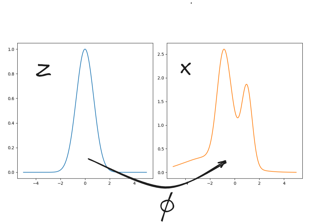
Back in 2015 when the world was young and Chat-GPT had not yet said its first words, a solution to sampling from complicated high-dimensional distributions arose: We can sample data from a multi-dimensional Gaussian and transform that Gaussian such that the resulting distribution matches some desired distribution.
How do we do this?
By using a simple change in variables! Say we sample \(z \sim \mathcal{N}\), and from \(z\) generate a random variable \(x\) by applying some invertible function \(\phi\) as \(x= \phi(z)\). How should \(p_x\) look like? We know that for every \(V \subset \mathbb{R}^d\) the following must hold
\[\mathbb{P}[x \in V] = \int_V p_x(x) dx = \int_{\phi^{-1}(z)} p_x(\phi(z))\mathrm{det}|\frac{d \phi}{dz}| dz = \int_Z p_z(z)dz \implies \\p_x(x) = p_z(z) \mathrm{det}|\frac{d \phi^{-1}}{dx}|\]The issue now becomes that we do not know what \(\phi\) should look like, so why don’t we learn it?
This is exactly what we will do, however we need to make sure that \(\phi_\theta\) (note that \(\phi\) is assigned some learnable parameters \(\theta\)) stays invertible.
As any mathematician worth their salt know that a composition of invertible functions is also invertible so if we decide on making \(\phi_\theta\) a neural network we only need to ensure that each layer is invertible! See more on how to do that here , but the crux is that our model has the following form:
\(\phi_{\theta} = f_k \circ f_{k-1}\circ ... \circ f_{2} \circ f_{1}\) Where \(f_i\) is the \(i\)-th layer of a neural network. It turns out this gives as plenty of nice properties:
-
The loss function is a simple log-likelihood
\(\mathcal{l}_{\theta,i} = \log p_{x_i} = \log p_z(z_i) + \sum_k \log |\frac{\partial f_k^{-1}}{\partial f_{k-1}}|(z_i)\) Where \(f_0 = z\). - We can use the network to sample \(x\) by first sampling \(z\) and passing it through the network.
- We can infer the likelihood of \(x\) by calculating the inverse of each layer and getting \(z\). According to property 1. calculating the log-likelihood is straightforward.
As with everything in life there is no such thing as free lunch, it turns out that by enforcing invertiblitly of network layers and the feasibility of calculating the Jaccobian of each layer \(\partial_{f_{k-1}} f_k^{-1} (z_i) \) severely limits the design choices and capability of the model. Therefore, the field was somewhat abandoned until 2024 when TarFlow came out, again showing how they are capable generators. Nevertheless, more recent research focused on a different approach on molding simpler distributions into more complicated ones, and one of the most prominent ones are based on flow matching.
2. Flow Matching
The main conceptual leap between older methods such as normalizing flows and flow matching is that while normalizing flow try to train a neural network to directly model the process of distribution molding in one step, flow matching trains the neural network to do that in many steps.
Again, let’s assume we have two random variables $Z$ and $X$ each sampled according to their respective distributions \(Z \sim p_z\) and \(X \sim p_x\), and we want to design a map from \(p_x\) to \(p_z\) (here we slightly deviate from the previous notation, now z will represent the data). Instead of moving \(p_x\) to \(p_z\) in one step let’s try to do this continuously by moving each \(X\sim p_x\) along a path
\[\psi_t: [0,1]\times \mathbb{R}^d \longrightarrow \mathbb{R}^d\]Such that \(\psi_0(x) = x \; \forall x \sim p_x\) and \(\psi_1(x)\sim p_z\). We call \(\psi_t\) a flow or probability path interchangeably.
Furthermore, at arbitrary \(t\) we get
\[X_t = \psi_t(X_0)\]which defines a velocity filed as
\[\frac{d X_t}{dt} = u_t(X_t)\]This can be expressed by a flow function \(\psi\) which satisfies
The result is that at each time step \(t\), \(\psi_t\) defines a new probability density function \(p_t(x)\). Furthermore we can relate \(u_t\) to \(p_t\) using the following continuity equation
\[ \partial_t p_t(x) + \nabla \cdot \big(p_t(x)u_t(x)\big )=0 \]What we want the neural network to learn is not \(\psi_t\) itself, rather we want it to learn the velocity field \( u^\theta _t (x) \). That is we minimize
\[\mathcal{L}_{FM}(\theta) = \mathbb{E}_{x\sim p_t(x)\; t\sim\mathcal{U}}\Big[\vert \vert u_t(x) - u^\theta_t(x)\vert \vert^2\Big]\]Once we have that we would sample an \(x\sim \mathcal{N}\) use that as the initial condition to integrate:
\[\frac{d X_t}{dt} = u^{\theta}_t(X_t)\]While this seems all to simple, it is not clear how would we get this \(u_t\), because if we had known it there would be no need to learn it with a neural network.
2.1 Conditional Flow matching - Constructing a target
Aside from the problem that we do not know what \(u_t(x)\) is we also do not know what \(p_z = p_{data}\) is, rather we only have access to a data set \(\mathcal{D}\) with a hopefully large enough sample drawn from the true distribution \(p_z\).
For the time being let’s try to solve a much simpler problem, where we have only one example in our dataset \(z_0 \in \mathcal{D}\). If that were the case we know the distribution \(p_z= \delta(z-z_0)\), and we know that we have to map each \(x\sim p_x\) to the same \(z_0\).
Even in this simplest of cases we are met with a choice; there are infinite probability paths \(\psi_t\) and \(u_t\) that would map from \(p_0\) to \(p_{data}\).
As usual we try to make use of Gaussian distributions in the following way
\[p_t(x) = \mathcal{N}(\alpha_t z_0,\beta_t^2)\]Where \(\alpha_t\) is a monotonically increasing function with \(\alpha_0=0\) and \(\alpha_1 = 1\), and \(\beta_t\) a monotonically decreasing function with \(\beta_0=1\) and \(\beta_1=0\). This makes sense because at \(t=0\) we end up with \(p_{x_0} = \mathcal{N}(0,1)\) and with \(p_{x_1} = \delta(z-z_0)\). We call this the Gaussian probability path. Furthermore typical choices for are
\[\alpha= t \\ \beta=1-t\]This now fully defines \(x_t(x)\) as
\[x_t =\psi_t(x_0)= \alpha_t z_0 + \beta_t x_0\;\; x_0\sim\mathcal{N}\]After a short derivation we end up with \(u_t(x_0) = \Big(\dot{\alpha_t} - \frac{\dot{\beta_t}}{\beta_t}\alpha_t \Big)z_0 + \frac{\dot{\beta_t}}{\beta_t}x_0\)
Plugging in our choices of \(\alpha_t = t\) and \(\beta = 1-t\) we get an incredibly simple expression for our target flow velocity
\[u_t(x_0) = z_0 - x_0 =u_t(x\vert z_0)\]But why would we even care for such a result? It seems obvious that there is no use in doing this if we have only a single data point in our dataset, so why do it?
The utility of this expression stems from the fact that we don’t know the distribution of data \(p_z\), rather we can only sample some batch \( \big(z_i \big) \) from the dataset, and in that scenario a more formal view reveals several important details to our approach:
- Since we’re sampling data we do not have access to the real \(u_t(x)\) and \(p_t(x)\), instead we have access to \(u_t(x\vert z)\), and \( p_t(x\vert z)\). That is we can only obtain a target for a conditional flow, and conditional probability path.
- Once some \(z_i\) has been sampled from the dataset the most unbiased estimator of the data distribution is that it is \(p(z \vert z_i) = \delta(z-z_i)\).
- Step 2. is especially important since we’ve done a nice derivation for the case \(p(z\vert z_0) = \delta(z-z_0)\), but more importantly by averaging over the dataset we can obtain the exact distribution \(p(z) = \int p(z_i) \delta(z-z_i) dz_i\)
Recall the continuity equation
Now that we’ve established the slight difference between the actual flow velocity \(u_t(x)\) and the conditional flow velocity \(u_t(x\vert z)\) our loss function changes to
\[\mathcal{L}(\theta)_{CFM} = \mathbb{E}_{z\sim p_{data}\; x\sim p_t(x\vert z)\;t\sim\mathcal{U}}\big[ \vert \vert u_t(x\vert z) - u^{\theta}_t(x)\vert \vert^2 \big]\\= \mathbb{E}_{z\sim p_{data}\; x\sim p_t(x\vert z)\;t\sim\mathcal{U}}\big[\vert \vert z-x -u_t^\theta(x)\vert \vert^2\Big]\]But wait! We are no longer fitting the model to the real \(u_t(x)\), rather to the conditional \(u_t(x\vert z)\), will this be good enough to fit to the model data?
In the next section we will discuss, a simple yet remarkable result as to why that is.
2.2 Conditional flow velocity
In the previous section we have only stated that there exists such a thing called the conditional flow velocity and that it is the thing we are regressing for, but how does it relate to the probability path and the real flow velocity?
Recall the probability continuity equation
\[\partial_t p_t(x) = - \nabla\cdot \big(p_t(x)u_t(x)\big)\quad (1)\]It should hold for any probability distribution, and so it should also hold for a conditional distribution
\[\partial_t p_t(x\vert z) = - \nabla\cdot \big(p_t(x\vert z)u_t(x\vert z)\big ) \quad (2)\]This is where the conditional flow velocity \( u_t(x\vert z) \) naturally occurs. As you might know, we can always marginalize a distribution according to w.r.t. random variable \( p(x) = \int p(x \vert z)p(z)dz \)
So let’s perform the marginalization of equation (1)
\[\partial_t p_t(x)=\partial_t \int p_t(x\vert z)p(z)dz = \int \partial_t p_t(x\vert z)p(z)dz = - \int \nabla\cdot \big(p_t(x\vert z)u_t(x\vert z)\big )p(z)dz\] \[=-\nabla \cdot p_t(x) \int u_t(x\vert z) \frac{p_t(x\vert z)p(z)}{p_t(x)} dz = \partial_tp_t(x)\\ \implies u_t(x) = \int u_t(x\vert z) \frac{p_t(x\vert z)p(z)}{p_t(x)} dz \qquad (\ast)\]The result \((\ast)\) finally relates the real flow velocity to the conditional flow velocity, and this result will be important to prove the following statement.
Theorem 1.
The original loss function
\[\mathcal{L}_{FM}(\theta) = \mathbb{E}_{x\sim p_x\; t\sim\mathcal{U}}\Big[\vert \vert u_t(x) - u^\theta_t(x)\vert \vert^2\Big]\]and the conditional loss function
\[\mathcal{L}(\theta)_{CFM} = \mathbb{E}_{z\sim p_{data}\; x\sim p_t(x\vert z)\;t\sim\mathcal{U}}\big[ \vert \vert u_t(x\vert z) - u^{\theta}_t(x)\vert \vert^2 \big]\]have the same gradients, and therefore the same local minima w.r.t. the model parameters \(\theta\).
Proof: The Flow Matching loss decomposes into three terms, where only two of them depend on \(\theta\), and the remaining is a constant w.r.t. \(\theta\)
\[\mathcal{L}_{FM}(\theta) = \mathbb{E}_{x\sim p_t(x\vert z) \, z\sim p_z \,t\sim\mathcal{U}}\Big[\vert \vert u_t(x) - u^\theta_t(x)\vert \vert^2\Big] \\ =\mathbb{E}\Big[u^\theta_t(x)^2 - 2 u_t(x) \cdot u_t^\theta(x) + u_t(x)^2 \Big] \\ = \mathbb{E}\Big[ u^\theta_t(x)^2 \Big] - 2\mathbb{E}\Big[ u_t(x) \cdot u_t^\theta(x) \Big] + C_1 \qquad (3)\]as have a closer look at the second term
\[\mathbb{E}{}\Big[ u_t(x) \cdot u_t^\theta(x) \Big] = \int dt \int dx \, p_t(x) u^\theta_t(x) \cdot u_t(x) =^{(\ast)} \int dt \int dx \int p_t(x) u_t^{\theta}(x) \cdot \int u_t(x\vert z) \frac{p_t(x\vert z)p(z)}{p_t(x)} dz\] \[= \int dt \int dx \int dz \; u_t^\theta(x) \cdot u_t(x\vert z) p(x\vert z)p(z) = \\ =\mathbb{E}_{x\sim p(x\vert z)\, z\sim p_z\, t\sim \mathcal{U}}\Big[u^\theta_t(x)\cdot u_t(x\vert z) \Big] \quad (4)\]We can substitute result (4) into equation (3), and add and subtract \(\mathbb{E}_{x\sim p_t(x\vert z)\,z\sim p_z\,t\sim \mathcal{U}}\Big[ u_t(x\vert z)^2\Big]\), (which is a constant w.r.t. \(\theta\)) to get
We define \(C_2\) as
\[C_2 = \mathbb{E}_{x\sim p_t(x\vert z)\,z\sim p_z\,t\sim \mathcal{U}}\Big[ u_t(x\vert z)^2\Big]\]The following expression follows trivially
\[\mathcal{L}_{FM}(\theta) = \mathbb{E}\Big[ u^\theta_t(x)^2 \Big] - 2\mathbb{E}\Big[ u_t(x\vert z) \cdot u_t^\theta(x) \Big] + \mathbb{E}\Big[ u_t(x\vert z)^2\Big] -\mathbb{E}\Big[ u_t(x\vert z)^2\Big] + C_1=\\ = \mathcal{L}_{CFM} + C_1 -C_2\] \[\nabla_{\theta} \mathcal{L}_{FM} = \nabla_{\theta} \mathcal{L}_{CFM}\]Q.E.D.
The result given by Theorem 1 tells us something remarkable, that we can use the extremely simple conditional flow velocity \(u_t(x\vert z) = z-x\), and still achieve the desired flow between the distribution \(p_0 = \mathcal{N}\) and \(p_1 = p_{data}\).
To recap the full procedure for training a flow matching model is:
- We define and initialize our model \(u_t^\theta\)
- We prepare our dataset \(\mathcal{D}\)
- We sample \(z\sim \mathcal{D}, x_0 \sim \mathcal{N}\), and \(t \sim \mathcal{U}\)
- We calculate the \(x_t\) via interpolation \(x_t = tz + (1-t)x_0\)
- We pass both \(x_t\) and \(t\) to the model to get the conditional flow velocity
- We calculate the target conditional flow velocity as \(u_t(x\vert z) = z - x_0\)
- We calculate the loss \(\mathcal{L}_{CMF}=\vert\vert u^\theta_t(x) - u_t(x\vert z)\vert\vert^2\) and back-propagate.
Once the model is trained we can sample new data in the following way:
- Sample \(x_0 \sim \mathcal{N}\), initialize the temporal grid \(T \subseteq [0,1]\)
- Perform numerical integration of \(u_t^\theta(x)\) along \(T\), with \(x_0\) as initial conditions.
3. Optimal Transport Flow Matching
So far we’ve overlooked one property of our trained flow matching model. While it does generates satisfactory samples and target distribution, it seems as if the samples are tracing a way longer path than necessary. This is due to random sampling.
In the image below we try to map samples from the left piles to the right piles, and a typical sample pairing between initial and target samples. Since we are training the model in a mini-batch manner we may pair initial samples from the top pile to the target samples from the bottom pile (and vice versa). This will train the model to trace a longer pile than necessary.
On the image below on the right you can see the learned sample paths. This hinder the models performance significantly.
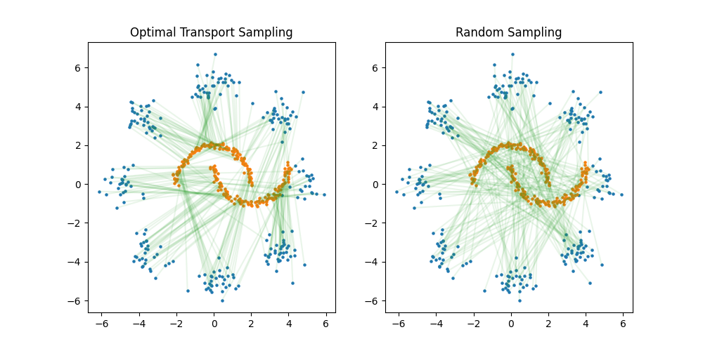
Image from Cambridge - An Introduction to Flow Matching
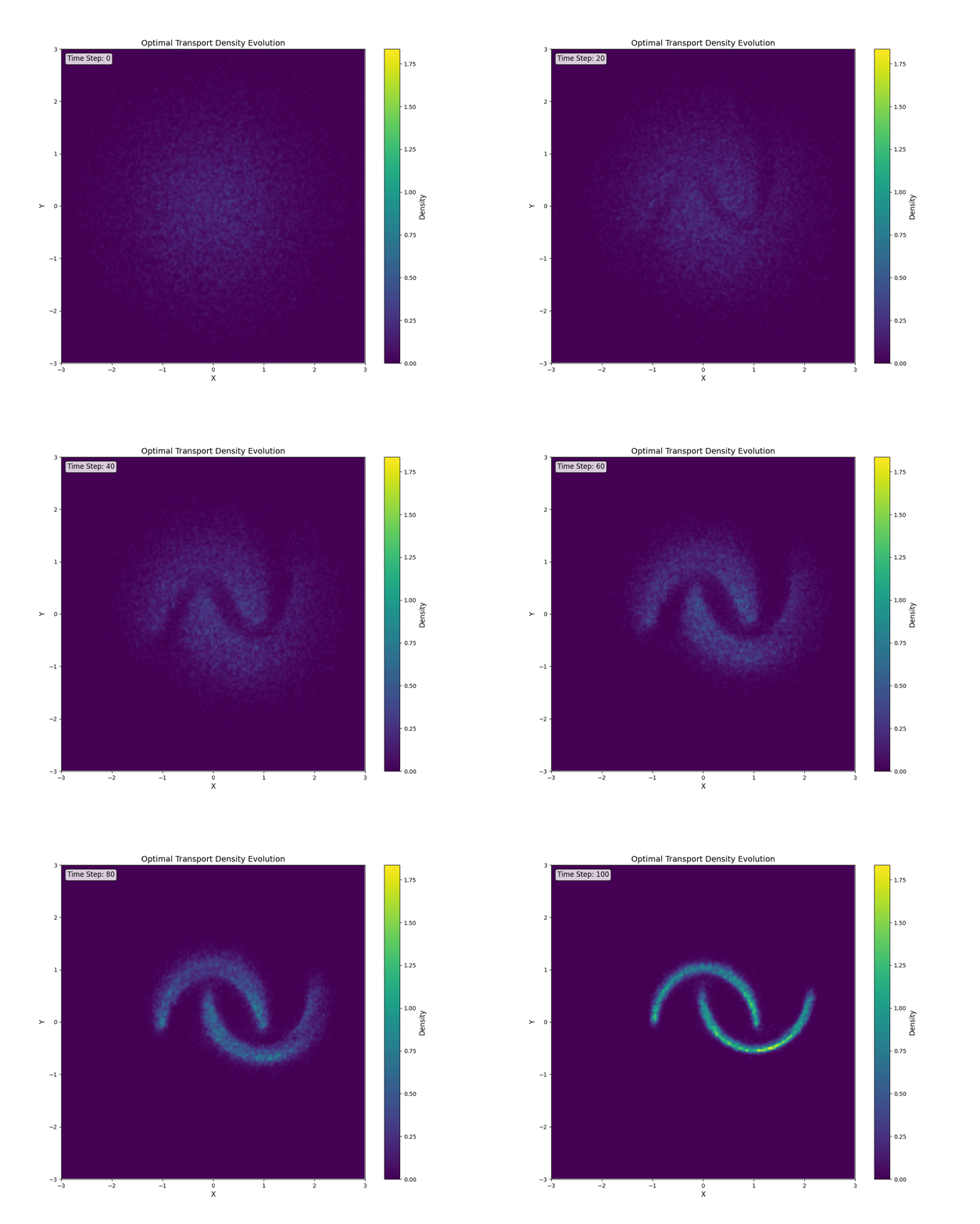
To avoid this, Mini-Batch Optimal Transport Sampling is employed. In the image below we try to map 8 symmetric Gaussians to the Two Moons. The image on the left shows target which batch pairs random sampling generates, while on the right you can see pairs generated by optimal transport sampling.
3.2 Comparison - Two Moons
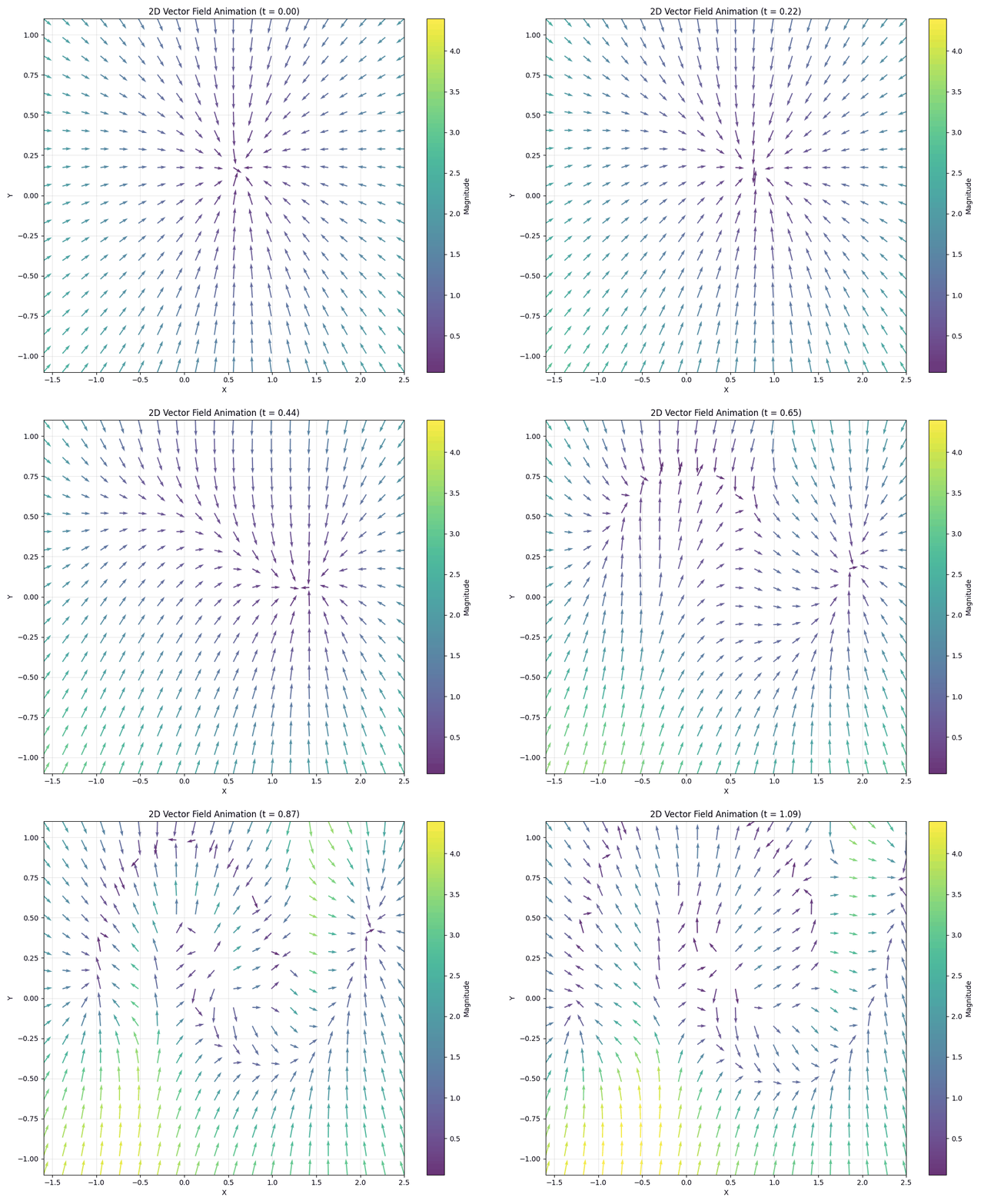
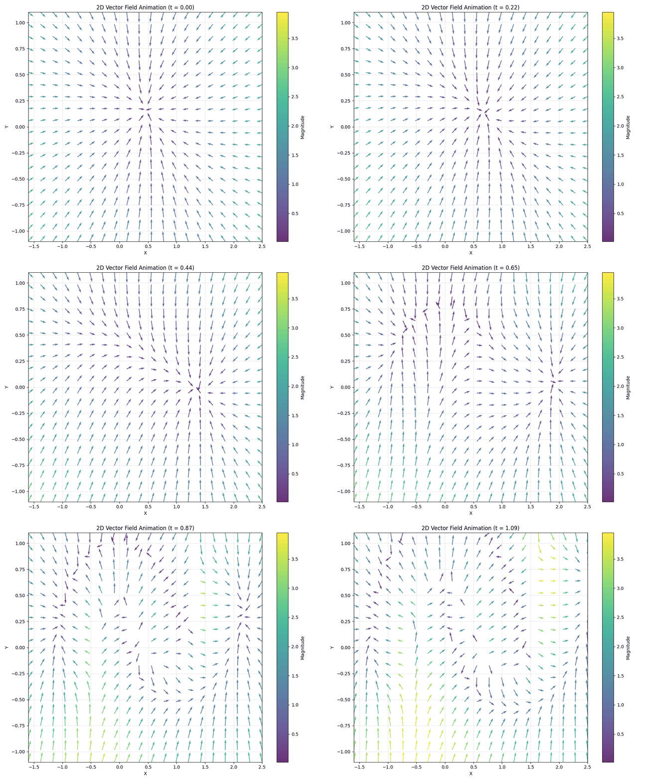
Regular Flow Velocity Field
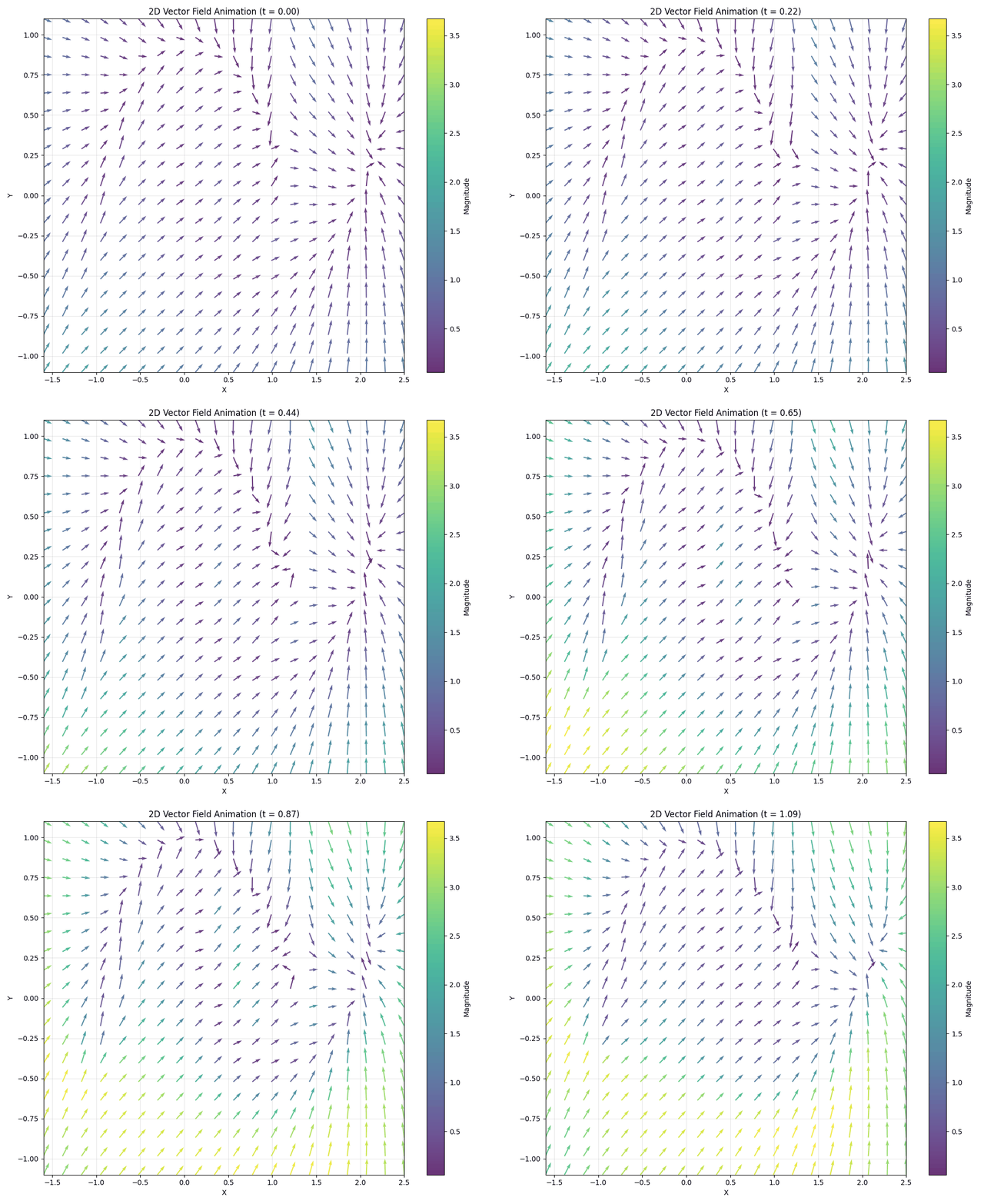
Optimal Transport Velocity Field
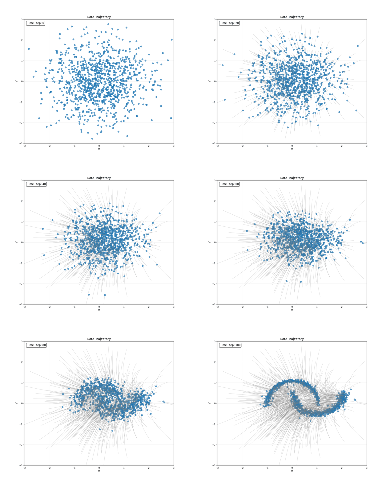
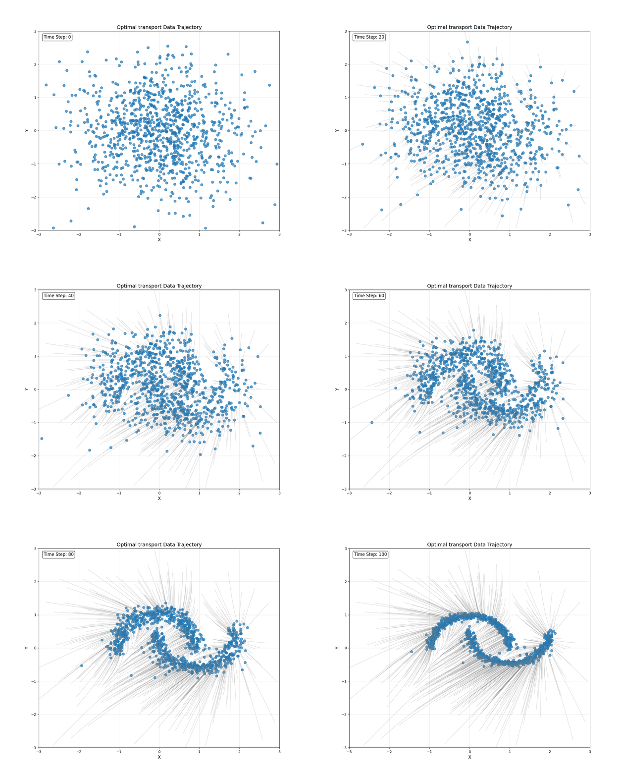
Regular Sample Trajectory
Optimal Transport Sample Trajectory
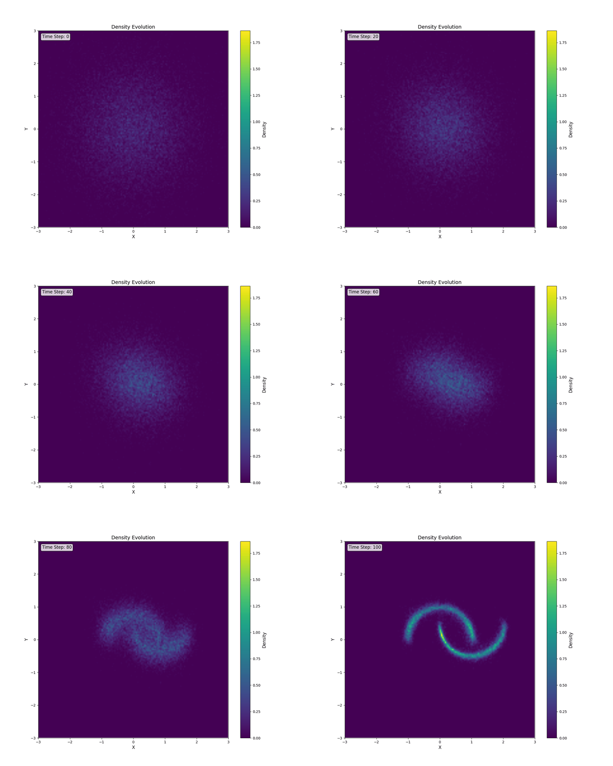
Regular Probability Density Evolution
Optimal Transport Probability Density Evolution
Resources
- MIT Lectures Page
- Literature
tags: [flow matching, generative modeling, deep learning, optimal transport]